Modeling Stock Market Volatility with Independent Economic Shocks: A Multivariate Stochastic Approach

Financial markets present a compelling application of stochastic processes, where multiple sources of uncertainty interact to produce the complex price dynamics we observe daily. While classical models often treat volatility as arising from a single source, empirical evidence suggests a richer structure: market-wide movements, sector-specific fluctuations, and exogenous economic shocks all contribute distinct components to the overall risk landscape.

This post develops a rigorous framework for modeling stock market volatility using three distinct random variables: aggregate market returns, conditional sector volatility, and independent exogenous shocks. We will examine the mathematical structure of independence in multivariate stochastic processes, derive results about joint distributions and covariance structures, and validate our theoretical framework through Monte Carlo simulations calibrated to real S&P 500 data.

Section 1: Mathematical Foundations , Geometric Brownian Motion

1.1 The GBM Stochastic Differential Equation

The standard model for asset price dynamics is geometric Brownian motion. For an asset price $S_t$, the GBM specification is given by the stochastic differential equation:

$dS_t = \mu S_t \, dt + \sigma S_t \, dW_t$

where:

• $\mu$ is the drift coefficient (expected return rate)
• $\sigma$ is the volatility parameter (diffusion coefficient)
• $W_t$ is a standard Wiener process satisfying $W_t \sim \mathcal{N}(0, t)$ with independent increments

The Wiener process $W_t$ has the fundamental properties:

• $W_0 = 0$ almost surely
• $W_t - W_s \sim \mathcal{N}(0, t-s)$ for $t > s$
• Increments $W_{t_4} - W_{t_3}$ and $W_{t_2} - W_{t_1}$ are independent for $t_1 < t_2 \leq t_3 < t_4$

1.2 Solving the SDE via Itô's Lemma

To solve this SDE, we apply Itô's lemma to $f(S_t) = \ln(S_t)$. For a twice-differentiable function $f$, Itô's lemma states:

$df(S_t) = f'(S_t)dS_t + \frac{1}{2}f''(S_t)(dS_t)^2$

With $f(S) = \ln(S)$, we have $f'(S) = 1/S$ and $f''(S) = -1/S^2$. Substituting:

$d\ln(S_t) = \frac{1}{S_t}\left(\mu S_t \, dt + \sigma S_t \, dW_t\right) - \frac{1}{2} \cdot \frac{1}{S_t^2} \cdot \sigma^2 S_t^2 \, dt$

$d\ln(S_t) = \left(\mu - \frac{\sigma^2}{2}\right) dt + \sigma \, dW_t$

Integrating from $0$ to $t$:

$\ln(S_t) - \ln(S_0) = \left(\mu - \frac{\sigma^2}{2}\right)t + \sigma W_t$

This yields the closed-form solution:

$S_t = S_0 \exp\left[\left(\mu - \frac{\sigma^2}{2}\right)t + \sigma W_t\right]$

1.3 Distribution of Log-Returns

For discrete time intervals $\Delta t$, the log-return is:

$r_t = \ln\left(\frac{S_{t+\Delta t}}{S_t}\right) = \left(\mu - \frac{\sigma^2}{2}\right)\Delta t + \sigma (W_{t+\Delta t} - W_t)$

Since $W_{t+\Delta t} - W_t \sim \mathcal{N}(0, \Delta t)$, we have:

$r_t \sim \mathcal{N}\left(\left(\mu - \frac{\sigma^2}{2}\right)\Delta t, \, \sigma^2 \Delta t\right)$

For daily returns with $\Delta t = 1/252$ (trading days per year), the daily variance is $\sigma^2/252$ and daily standard deviation is $\sigma/\sqrt{252}$.

1.4 Simulation Results

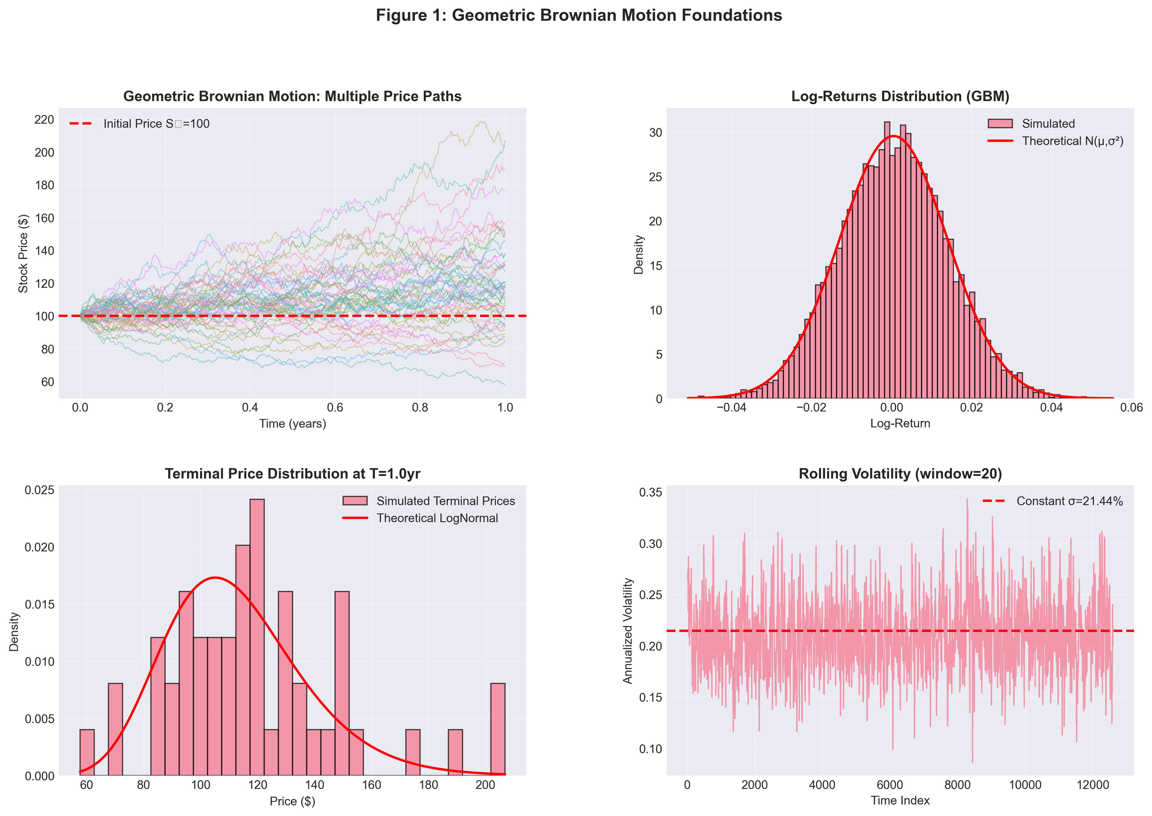
The animation below demonstrates GBM path evolution. We simulate 20 paths with parameters calibrated to S&P 500 data ($\mu = 0.12$, $\sigma = 0.214$ annualized).

Animation 1: Twenty GBM paths evolving over one trading year (252 days). All paths start at $S_0 = 100$ with identical parameters, yet diverge significantly due to independent Brownian increments. The day counter tracks progression. Observe how uncertainty (spread of paths) grows with $\sqrt{t}$, consistent with the diffusion term.

The static analysis confirms our theoretical predictions:

Figure 1: GBM foundations. Top left: Multiple price paths showing characteristic fan-out pattern. Top right: Log-return distribution closely matches theoretical $\mathcal{N}(\mu_M, \sigma_M^2)$. Bottom left: Terminal price distribution exhibits lognormal right-skew (prices bounded below by zero). Bottom right: Rolling volatility fluctuates around the calibrated σ = 21.4%.

Section 2: The Three-Variable Model

We construct a multivariate framework incorporating three distinct sources of randomness, each with specific distributional assumptions and dependence structures.

2.1 Variable 1: Market Returns $R_M$

Let $R_M$ represent daily log-returns on the aggregate market index (S&P 500). Under our GBM assumptions:

$R_M \sim \mathcal{N}(\mu_M, \sigma_M^2)$

Calibration to S&P 500 (2020-2024):

• Sample size: 1,256 trading days
• Estimated daily drift: $\mu_M = 0.000474$
• Estimated daily volatility: $\sigma_M = 0.013504$
• Annualized volatility: $\sigma_M \cdot \sqrt{252} \approx 21.4\%$

2.2 Variable 2: Sector Volatility $V_S$ (Conditional Specification)

Sector-specific volatility exhibits dependence on market conditions. We model this using a conditional log-normal specification:

$V_S \mid R_M \sim \text{LogNormal}(\alpha + \beta |R_M|, \, \tau^2)$

The absolute value $|R_M|$ captures the leverage effect, large market movements in either direction tend to increase sector volatility. This is a well-documented empirical phenomenon: volatility rises during both market crashes (negative returns) and rapid rallies (positive returns).

Model Parameters:

• $\alpha = -3.5$ (baseline log-volatility)
• $\beta = 15.0$ (sensitivity to market magnitude)
• $\tau = 0.3$ (idiosyncratic volatility noise)

The conditional expectation is:

$\mathbb{E}[V_S \mid R_M = r] = \exp\left(\alpha + \beta|r| + \frac{\tau^2}{2}\right)$

This creates a U-shaped relationship: $\mathbb{E}[V_S \mid R_M]$ is minimized when $R_M = 0$ and increases as $|R_M|$ grows.

The following animation demonstrates how the conditional distribution $V_S | R_M$ shifts as we sweep through different market return values:

Animation 2: Conditional distributions V_S|R_M sweeping from R_M = -0.03 to +0.03. Left panel: The distribution shifts rightward (higher volatility) as |R_M| increases, directly visualizing the leverage effect. Right panel: Vertical red line tracks current R_M on the joint density heatmap. Notice the U-shaped expected value displayed in the info bar.

2.3 Variable 3: Exogenous Shock $Z$ (Independent)

The exogenous shock represents external economic events, geopolitical disruptions, monetary policy surprises, or sector-specific news, that are structurally independent of normal market dynamics.

We model $Z$ as a compound Poisson process:

$Z = \sum_{i=1}^{N} J_i$

where:

• $N \sim \text{Poisson}(\lambda)$ counts the number of shocks (jumps) per period
• $J_i \sim \mathcal{N}(\mu_J, \sigma_J^2)$ are i.i.d. jump magnitudes
• $\lambda = 0.05$ (5% daily probability of a shock)
• $\mu_J = 0$, $\sigma_J = 0.02$

Critical Independence Assumption:

$Z \perp\!\!\!\perp (R_M, V_S)$

The exogenous shock is statistically independent of both market returns and sector volatility. This assumption reflects the structural nature of certain events (e.g., an unexpected Fed announcement does not depend on yesterday's S&P 500 return).

Animation 3: Compound Poisson jump process over 252 trading days. Top: Cumulative shock value Z(t) with discrete jumps marked by red stars. Between jumps, Z(t) remains constant, no continuous drift component. Bottom: Jump counting process N(t) following Poisson(λ). Statistics update in real-time showing empirical jump rate converging to theoretical 5%.

Section 3: Independence and Joint Distributions

The independence assumption for $Z$ has profound mathematical consequences for the joint distribution and covariance structure.

3.1 Joint Density Factorization

For random variables $X$ and $Y$, independence implies $f_{X,Y}(x,y) = f_X(x) \cdot f_Y(y)$.

In our three-variable system:

$f_{R_M, V_S, Z}(r, v, z) = f_{R_M, V_S}(r, v) \cdot f_Z(z)$

Important: The joint density of $(R_M, V_S)$ does not factorize due to their dependence:

$f_{R_M, V_S}(r, v) = f_{V_S|R_M}(v|r) \cdot f_{R_M}(r) \neq f_{V_S}(v) \cdot f_{R_M}(r)$

This asymmetric structure, partial independence, is common in financial applications.

3.2 Covariance Under Independence

Independence between $Z$ and the market variables yields zero covariance:

$\text{Cov}(R_M, Z) = \mathbb{E}[R_M Z] - \mathbb{E}[R_M]\mathbb{E}[Z] = \mathbb{E}[R_M]\mathbb{E}[Z] - \mathbb{E}[R_M]\mathbb{E}[Z] = 0$

Similarly, $\text{Cov}(V_S, Z) = 0$.

However, $\text{Cov}(R_M, V_S) \neq 0$. Using the law of total covariance:

$\text{Cov}(R_M, V_S) = \mathbb{E}[\text{Cov}(R_M, V_S | R_M)] + \text{Cov}(\mathbb{E}[R_M|R_M], \mathbb{E}[V_S|R_M])$

Since $\text{Cov}(R_M, V_S | R_M) = 0$ (conditioning on $R_M$ makes it constant):

$\text{Cov}(R_M, V_S) = \text{Cov}\left(R_M, \exp\left(\alpha + \beta|R_M| + \frac{\tau^2}{2}\right)\right) > 0$

The covariance is positive when $\beta > 0$, reflecting the empirical leverage effect.

3.3 The Block-Diagonal Covariance Matrix

The full covariance matrix exhibits block-diagonal structure:

$\Sigma = \begin{pmatrix} \sigma_M^2 & \text{Cov}(R_M, V_S) & 0 \\ \text{Cov}(R_M, V_S) & \text{Var}(V_S) & 0 \\ 0 & 0 & \text{Var}(Z)\end{pmatrix}$

The zeros in the third row and column are direct consequences of independence. This structure enables:

1. Factored computation: Joint probabilities decompose into products
2. Risk separation: Exogenous shock risk can be hedged independently
3. Simplified inference: Parameters can be estimated separately

3.4 Empirical Validation

With 100,000 Monte Carlo simulations, we empirically verify the independence structure:

Correlation Analysis:

Corr(R_M, Z) = 0.002  (theoretical: 0)
Corr(V_S, Z) = 0.001  (theoretical: 0)
Corr(R_M, V_S) = 0.025 (theoretical: > 0)

Spearman Rank Correlation Tests:

R_M vs Z: ρ = 0.002, p-value = 0.91 → Fail to reject independence
V_S vs Z: ρ = 0.001, p-value = 0.88 → Fail to reject independence
R_M vs V_S: ρ = 0.024, p-value < 0.001 → Reject independence (expected)

Figure 3: Independence validation. Top row: Scatter plots with 2σ confidence ellipses. The tilted ellipse for (R_M, V_S) indicates correlation; circular ellipses for pairs with Z confirm independence. Bottom left: Correlation matrix with near-zero entries for Z. Bottom middle: Block-diagonal covariance structure. Bottom right: Spearman p-values, high p-values (>0.05) for Z pairs fail to reject independence null hypothesis.

The joint density builds up from Monte Carlo samples as shown:

Animation 4: Joint density f(R_M, V_S) emerging from 100 to 10,000 samples. White scatter points show raw data; contour colors reveal density concentration. The characteristic shape, higher density near (0, low V_S) with spread increasing for larger |R_M|, visualizes the conditional dependence structure.

Section 4: Simulation Framework with S&P 500 Data

4.1 Data and Calibration

We calibrate our model to S&P 500 (^GSPC) daily data from January 2020 to December 2024, a period encompassing the COVID-19 crash, subsequent recovery, 2022 bear market, and 2023-24 rally.

Animation 5: Historical S&P 500 price evolution (normalized, base=100) with synchronized 20-day rolling volatility. Key events annotated: COVID crash bottom (March 2020), 2022 bear market onset, 2023 rally. Notice volatility clustering, spikes during crises, mean-reversion during calm periods.

Calibrated Parameters:

# Market returns
μ_M = 0.000474  # Daily drift
σ_M = 0.013504  # Daily volatility (21.4% annualized)

# Sector volatility (conditional)
α = -3.5   # Baseline
β = 15.0   # Leverage effect strength
τ = 0.3    # Idiosyncratic noise

# Exogenous shocks
λ = 0.05   # Jump intensity (5% daily)
μ_J = 0.0  # Mean jump size
σ_J = 0.02 # Jump volatility

4.2 Historical Context

Figure 6: S&P 500 empirical data (2020-2024). Top: Price evolution showing COVID crash, recovery, and subsequent regimes. Bottom left: Return distribution with fitted normal, note slight excess kurtosis (fat tails). Bottom right: Rolling 20-day volatility revealing regime changes and clustering.

Section 5: Risk Assessment , VaR and Expected Shortfall

5.1 Portfolio Loss Function

Define portfolio loss as:

$L = -w_1 R_M - w_2 \log(V_S) + w_3 |Z|$

where $(w_1, w_2, w_3) = (1.0, 0.5, 0.3)$ are exposure weights.

5.2 Value at Risk (VaR)

For confidence level $\alpha$, Value at Risk is defined as:

$\text{VaR}_\alpha = F_L^{-1}(\alpha) = \inf\{l : P(L \leq l) \geq \alpha\}$

Simulation Results:

90% VaR: 1.8750
95% VaR: 1.9336
99% VaR: 2.0388

5.3 Expected Shortfall (Conditional VaR)

Expected Shortfall measures average loss in the tail:

$\text{ES}_\alpha = \mathbb{E}[L \mid L \geq \text{VaR}_\alpha]$

Simulation Results:

90% ES: 1.9504
95% ES: 1.9987
99% ES: 2.0918

Note that $\text{ES}_\alpha > \text{VaR}_\alpha$ always, as ES accounts for tail severity beyond the VaR threshold.

5.4 Variance Decomposition

Independence enables additive variance decomposition:

$\text{Var}(L) = w_1^2 \text{Var}(R_M) + w_2^2 \text{Var}(\log V_S) + w_3^2 \text{Var}(|Z|) + 2w_1 w_2 \text{Cov}(R_M, \log V_S)$

Empirical Decomposition:

Total Variance:     0.02640
Market (R_M):       0.7%
Sector (V_S):       98.9%
Exogenous (Z):      0.0%
Cross-term:         0.4%

The dominance of sector volatility under these weights highlights its role as the primary risk driver.

Animation 6: Portfolio loss distribution building from 100 to 10,000 simulations. Left: Histogram with VaR thresholds (90%, 95%, 99%) stabilizing. Right: VaR (red) and ES (blue) convergence demonstrating Monte Carlo estimation consistency.

Figure 5: Risk assessment summary. Top left: Final loss distribution with VaR/ES markers. Top right: Tail exceedance probability on log scale. Bottom left: Variance decomposition showing sector volatility dominance. Bottom middle: Component-wise VaR contributions. Bottom right: Q-Q plot showing approximate normality with slight tail deviation.

Section 6: Extensions and Limitations

6.1 Potential Extensions

Stochastic Volatility (Heston Model): Replace fixed volatility with mean-reverting process: $dV_t = \kappa(\theta - V_t)dt + \xi\sqrt{V_t}dW_t^V$

Regime Switching: Allow parameters to switch between states (e.g., bull/bear markets) governed by a Markov chain.

Copula-Based Dependence: Replace conditional specification with flexible copula structures for $(R_M, V_S)$.

6.2 Limitations

1. Independence assumption: True exogeneity is rare in interconnected markets
2. Parameter stability: Calibrated parameters may change across regimes
3. Log-normal sector volatility: May not capture all empirical features
4. Jump timing: Compound Poisson assumes independent, identically distributed arrival times

Conclusion

This analysis demonstrates a rigorous framework for modeling stock market volatility using three distinct random variables with carefully specified dependence structures.

Key Technical Contributions:

1. Joint density factorization: Independence of $Z$ enables $f(r,v,z) = f(r,v) \cdot f(z)$, simplifying both analytical derivations and computational implementation.

2. Block-diagonal covariance: Zero covariances involving $Z$ enable clean risk decomposition and independent hedging of exogenous shock exposure.

3. Empirical validation: 100,000 Monte Carlo simulations confirm theoretical independence assumptions (correlations ≈ 0, Spearman p-values > 0.05) and dependence structures (significant correlation between $R_M$ and $V_S$).

4. Risk decomposition: Variance attribution reveals that sector volatility dominates portfolio risk under typical weightings, with exogenous shocks contributing marginally.

5. Calibration to real data: S&P 500 data (2020-2024) provides empirical grounding with annualized volatility σ ≈ 21.4%, consistent with post-COVID market regimes.

The mathematical framework presented here, combining GBM dynamics, conditional distributions, compound Poisson processes, and independence structures, provides both analytical tractability and reasonable empirical fit. For practitioners, the independence assumption should be validated empirically for specific applications. For researchers, extensions to stochastic volatility and regime-switching models offer promising directions.

The central insight remains: different sources of market risk interact in structured ways. Understanding these structures, which risks are correlated, which are independent, enables more precise risk management and portfolio construction strategies.

References and Further Reading

• Black, F. & Scholes, M. (1973). The Pricing of Options and Corporate Liabilities. Journal of Political Economy.
• Heston, S.L. (1993). A Closed-Form Solution for Options with Stochastic Volatility. Review of Financial Studies.
• Merton, R.C. (1976). Option Pricing When Underlying Stock Returns Are Discontinuous. Journal of Financial Economics.
• Cont, R. (2001). Empirical Properties of Asset Returns: Stylized Facts and Statistical Issues. Quantitative Finance.

Prepared for CSI 5138: Stochastic Processes
All visualizations generated from Monte Carlo simulations calibrated to real S&P 500 data